9. Studies section
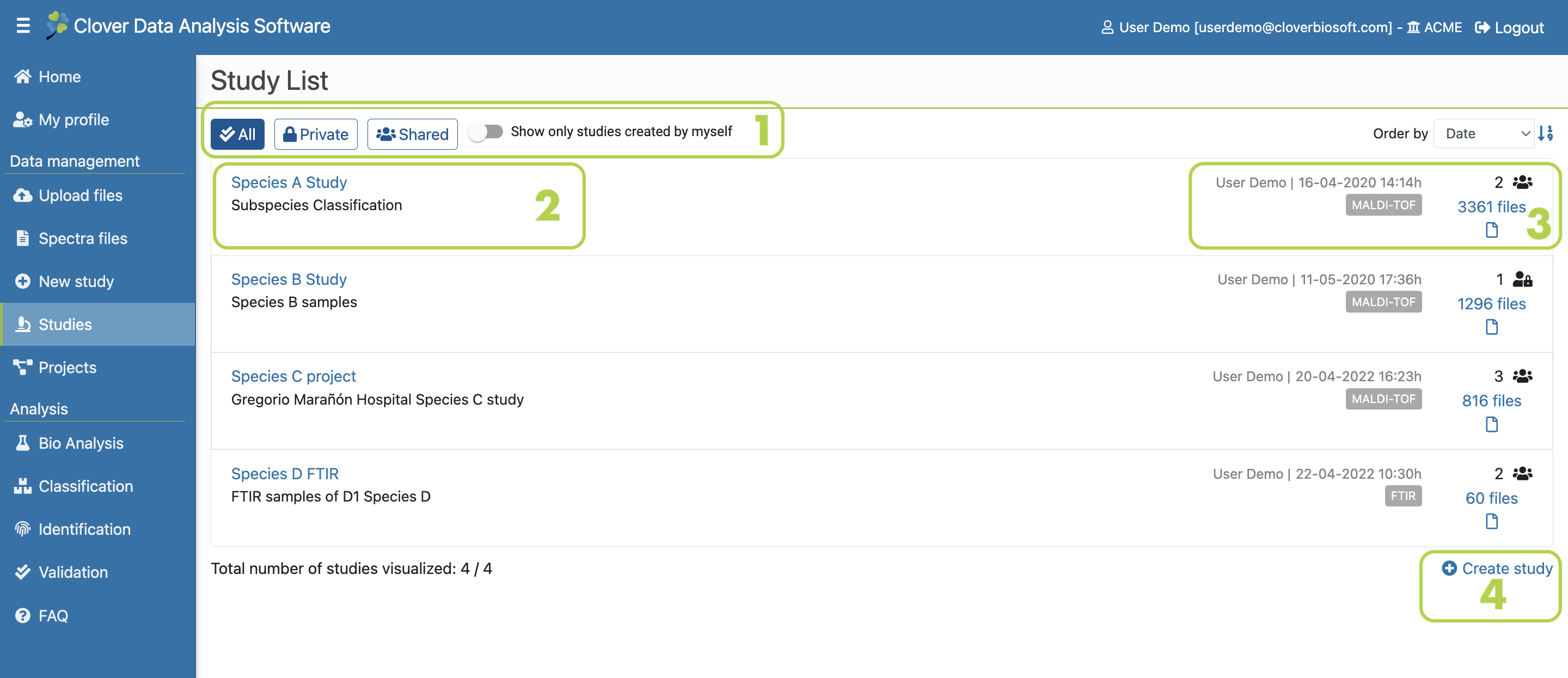
Figure 9.1: Studies section layout
Here, you can see your list of studies. You can organise them by private or shared studies (Figure 9.1-1). You can also filter this information by only showing the studies that you have created. The study data is indicated as follows in this section:
- The name and the description of the study. The name is also a link that will redirect you to a new layout with extensive information of the study (Figure 9.1-2).
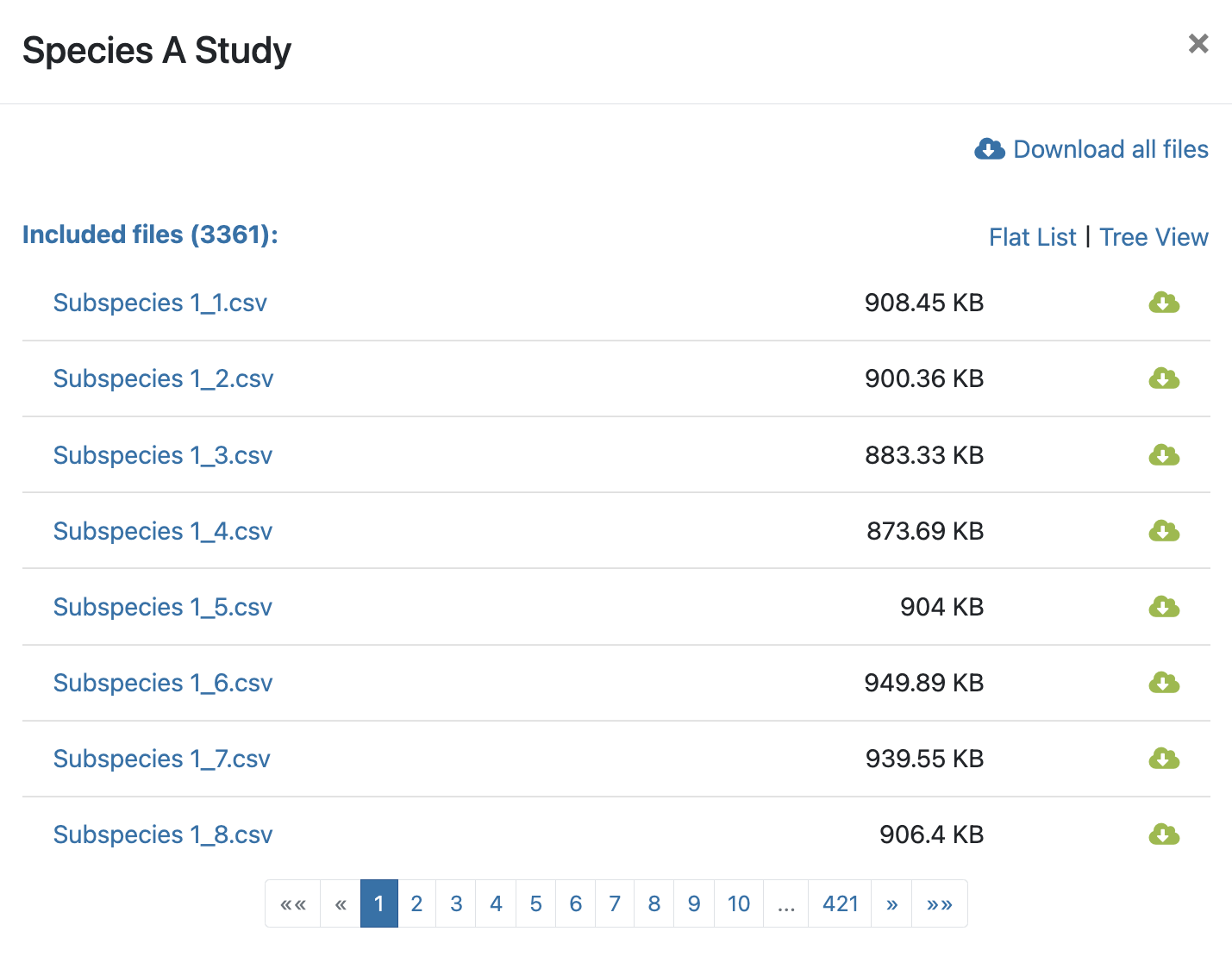
- The creator of the study and the creation date (Figure 9.1-3). The data source (MALDI-TOF or FTIR), the number of users with access to the study and the number of files that are part of the study are also displayed in this box. Click on the number of files to see detailed information about them. You can organise the information as a flat list or as a tree as well as download all or some of the files (Figure 9.2).
- It is possible to create a new study within this layout too by clicking on Create Study (Figure 9.1-4). This action will take you to the Studies section.
If no studies are created yet, this section displays just the option to create the first study.
Figure 9.2: Detailed information about the files of a study
9.1. Detailed study section
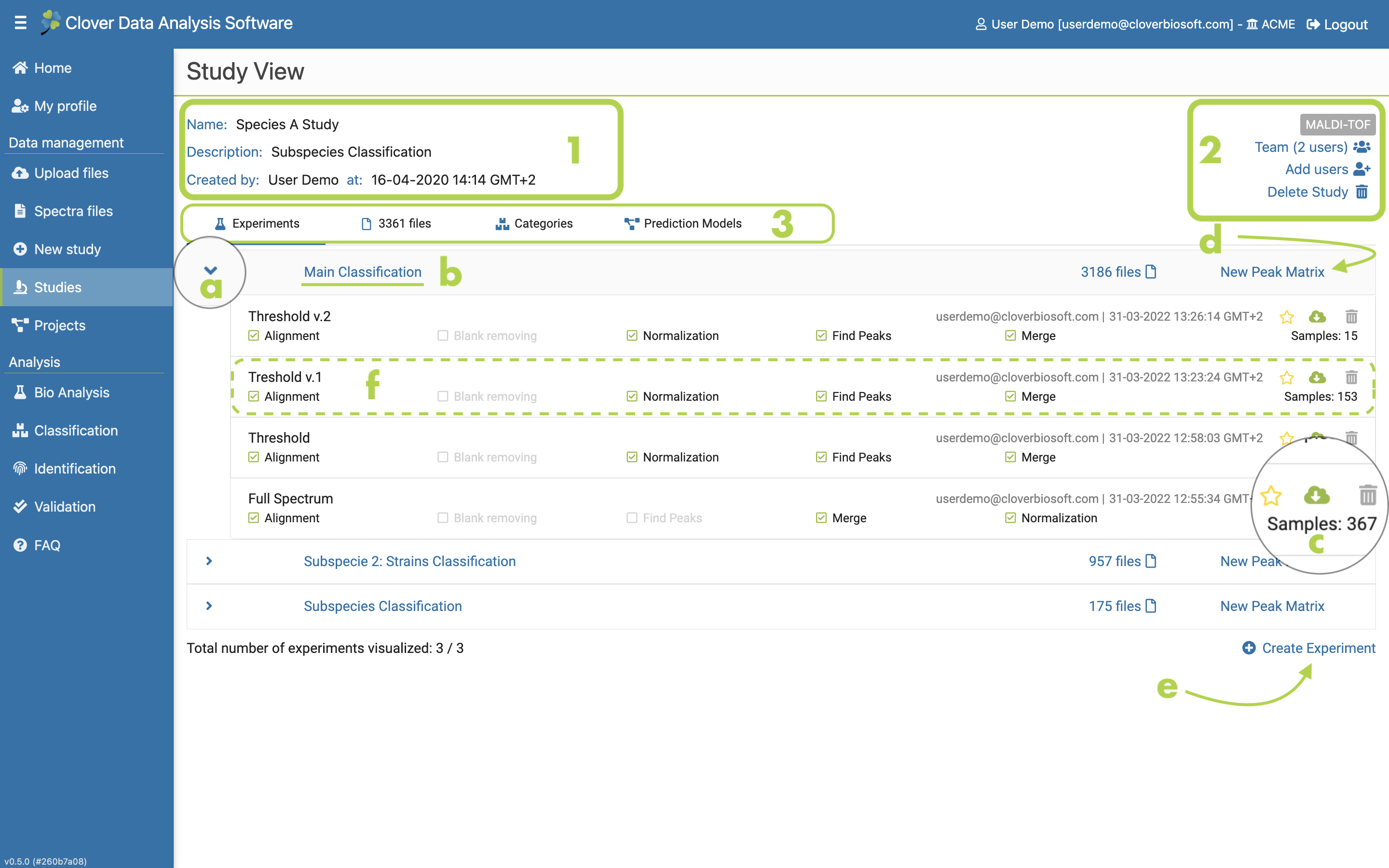
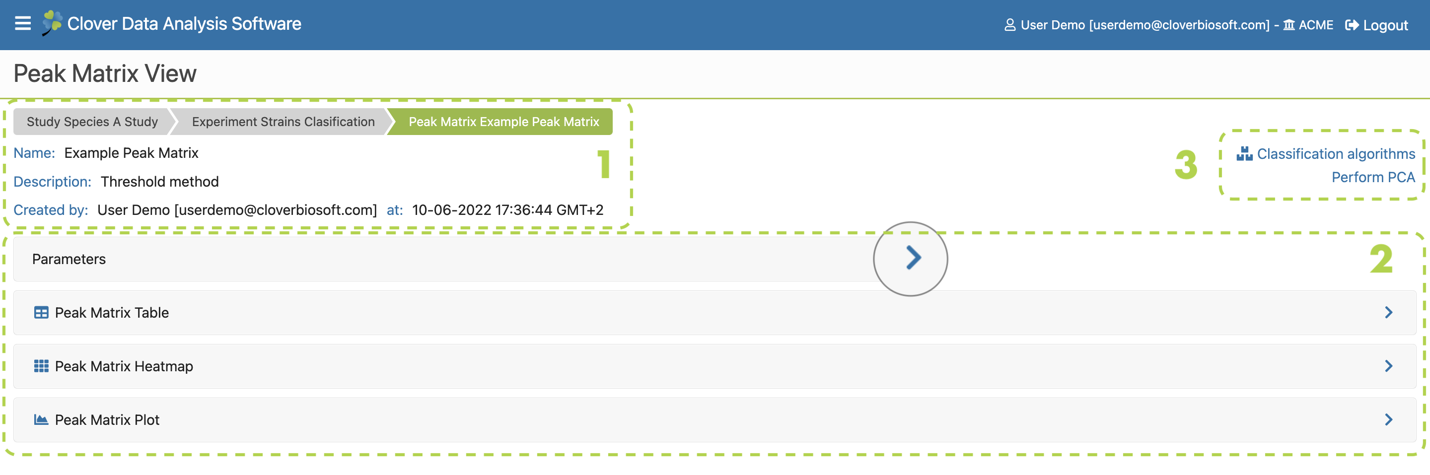
Figure 9.3: Detailed study layout with an experiment subsection that has various experiments with peak matrices
As mentioned before, if you click on the name of a study, a new layout will be displayed with all the study information. This is the main layout of the selected study, which contains all its information, data and options.
- General information of the study: name, description, creation date and owner of the study (Figure 9.3-1).
- Share and collaborative options (Figure 9.3-2).
- The data source (MALDI-TOF in this example).
- Team (x users). The number of users with access to the study. If you click there, the platform will display a new layout with the user information, i.e. email, name and organization (Figure 9.4).
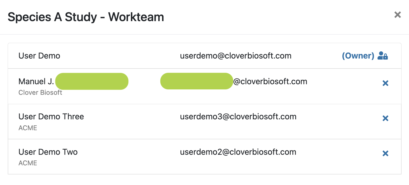
Figure 9.4: Detailed information about the users that are following a study
- Add Users. A new layout appears when clicking here. You can share the study with the coworkers of your organization just by selecting the box to the left of the user name or using the Select All button (Figure 9.5a). If the user you want to share the study with is out of your organization, you must select the With other option and write the registered email address of the user (Figure 9.5b).

Figure 9.5: Share Study form. a) Within your organization layout. b) With others users layout
- Delete Study. This option deletes all study content and configuration, but files will be still uploaded in their respective folder in the platform. The platform will advise you if you are sure to do it or if there is any conflict that prevent you to do it.
Please note that only studies created by yourself are susceptible to be deleted.
- Study content and metadata (Figure 9.3-3). These options will take you to their subsec- tions within the study (Figure 9.6). The Experiments subsection is displayed as preset. The list of experiments of a new study is empty at the beginning. You have to click on the here link to create a new one. This part will be explained in Experiment section later.

Figure 9.6: Study tabs detailed view
- Experiments. Tab with the list of experiments that are part of the study and their peak matrices. You can order the experiments by date or by name, and there is also a link for creating a new experiment.
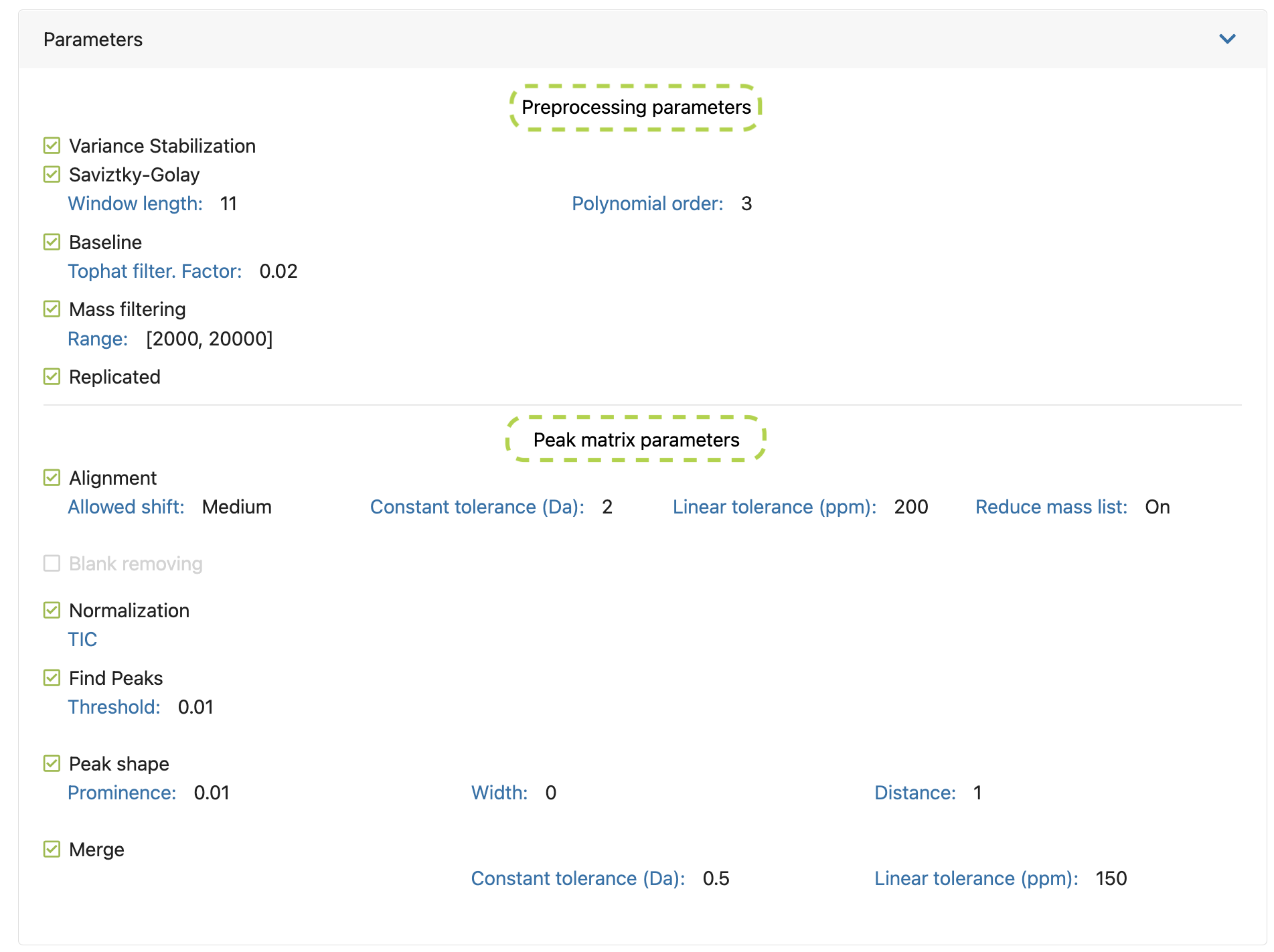
If you click on the left arrow next to the experiment name (Figure 9.3a), a dropdown will appear with the peak matrices created within that experiment and their main parameters. Detailed information about these parameters can be consulted placing the cursor above it (Figure 9.3-f). Furthermore, you can download, delete or mark as favourite any of your peak matrices (Figure 9.3c).
You can also go to the experiment subsection to amplify the information of the selected experiment by clicking on its name (Figure 9.3b). In the other hand, new peak matrices within the selected experiment or new experiments can be created directly in this subsection by clicking on New Peak Matrix (Figure 9.3-d) and Create Experiment (Figure 9.3-e) buttons respectively. Both processes will be described in Peak Matrix generation section and Experiment subsection as com- mented above.
- Files. Tab with the number of files included on the study. Click on it if you want to see more information about those files showed in the tree list view, or bring previously uploaded files to the study (Figure 9.7a) as well as remove folders or files from it (Figure 9.7c).
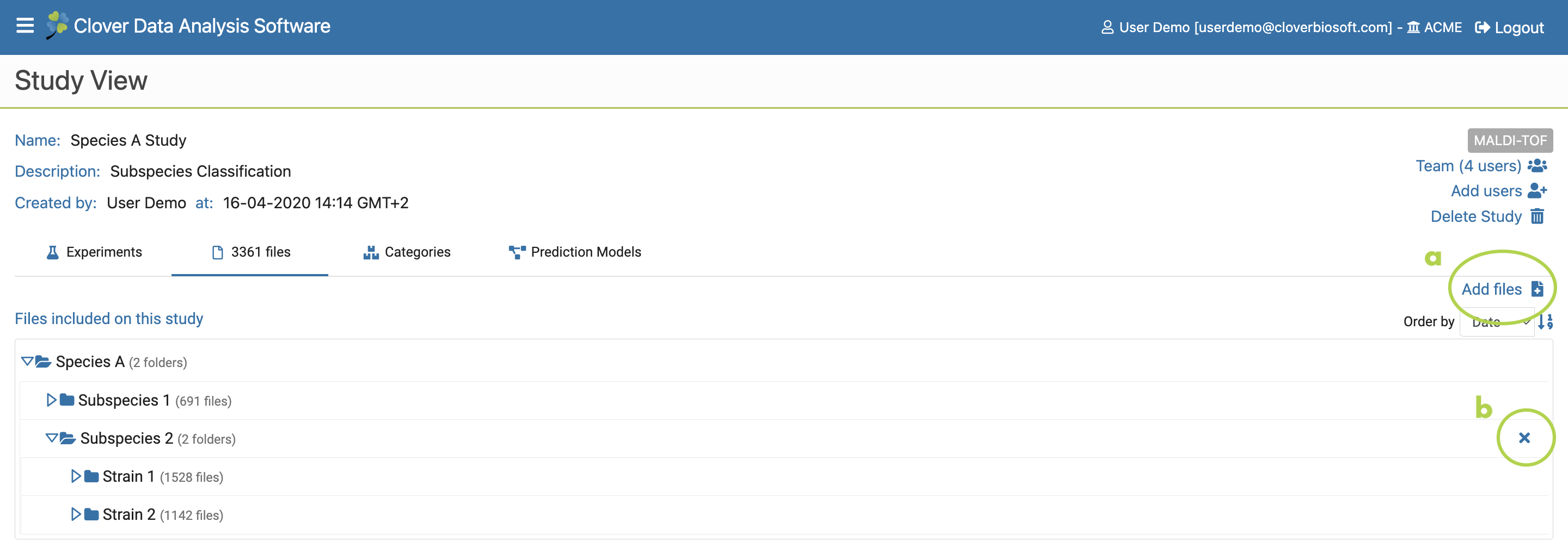
Figure 9.7: Files Subsection layout within Study View
Please note that only studies created by yourself are susceptible to be deleted.
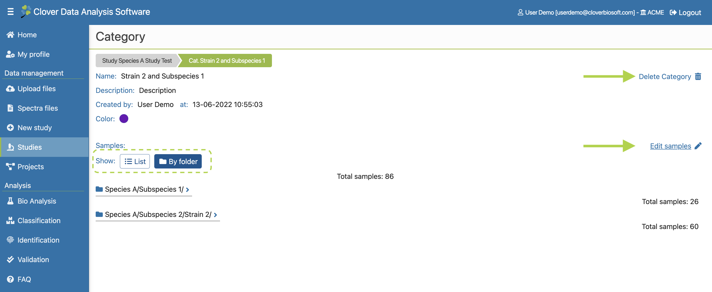
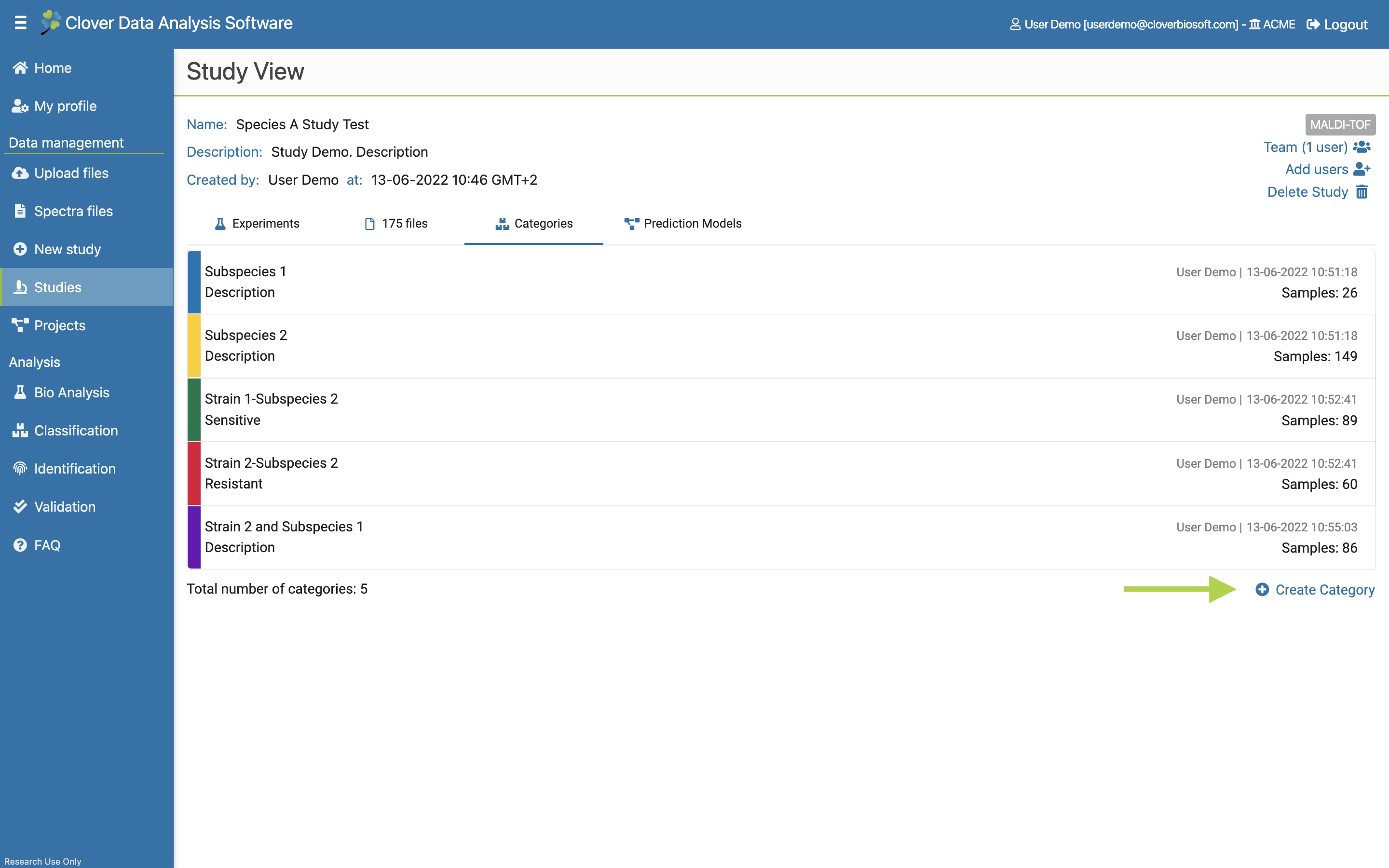
- Categories. Tab with the tools needed to create and manage the categories of the study. This tab will also be explained with more details in Categories subsection.
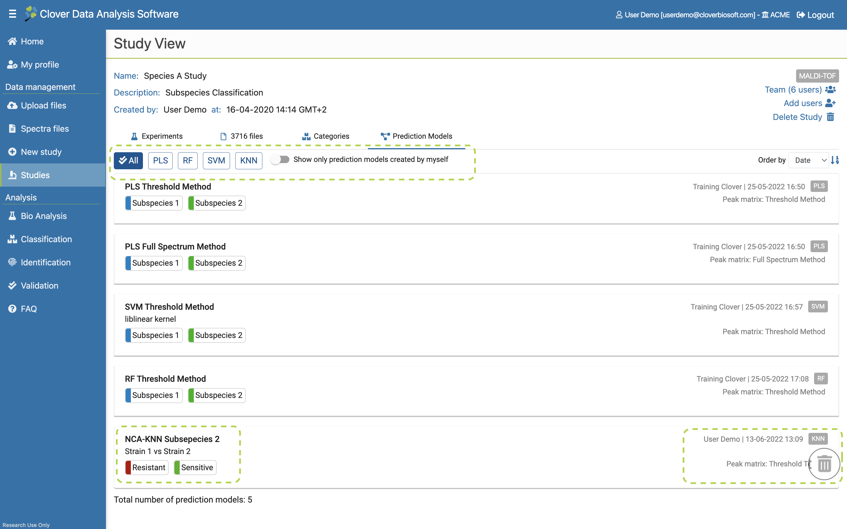
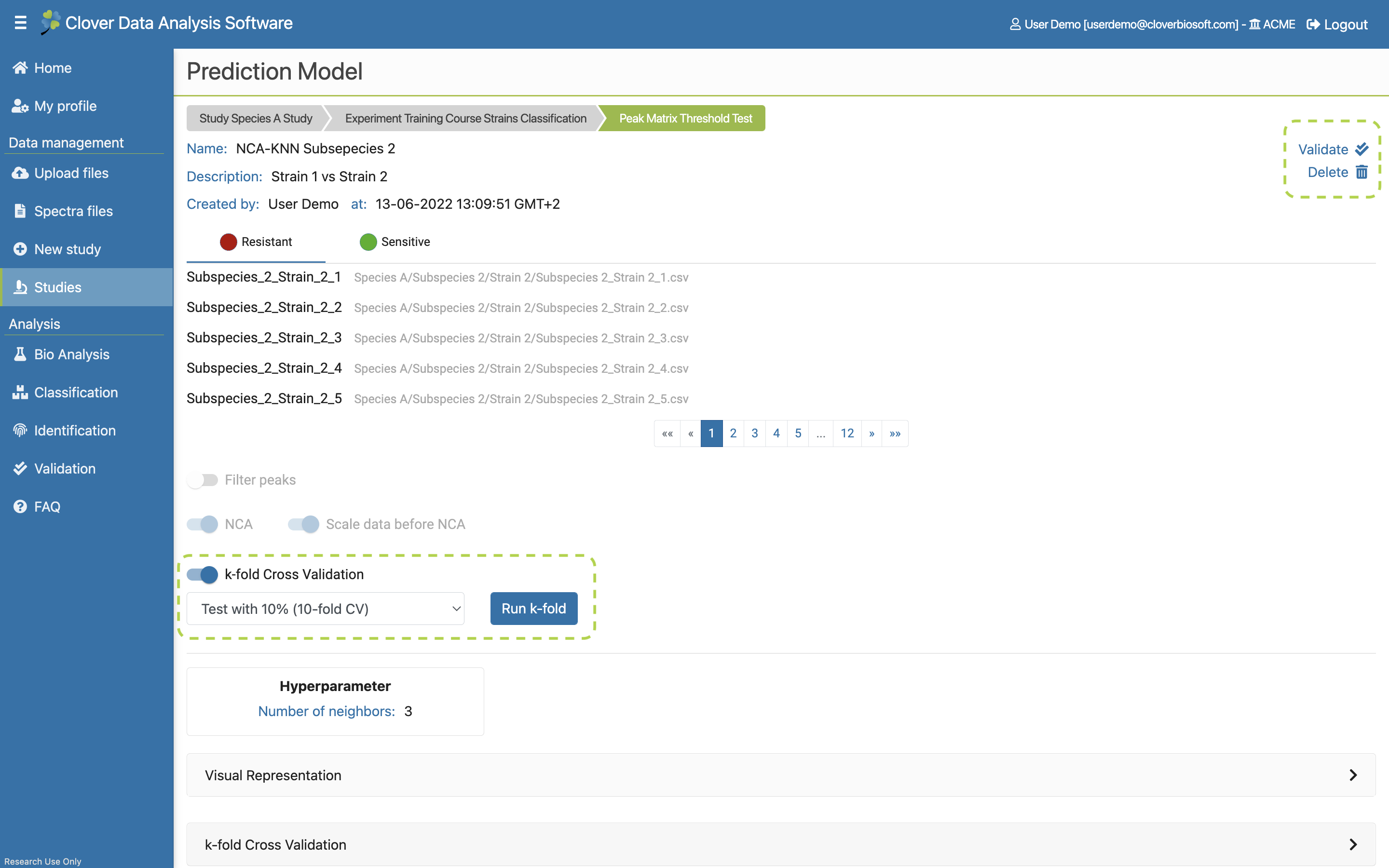
- Prediction Models. Tab with all Prediction models saved at the study. The results of algorithms can be saved as these prediction models. They can be validated and used for identifying new samples. This tab will be further explained in Prediction Model subsection.
9.2. New Experiment setp
After the study is created, you can create as many experiments within it as you need. For this, click on Next Experiment button in the Study View layout (Figure 9.3e), this action takes you to New Experiment step. This layout is pretty similar to the New study one (Figure 9.8). The only new thing here is the Experiment metadata. You can write whatever information you want here. Type in a key name and a value for it and press the Add button to add the pair to the experiment. Press the Save button to save your experiment.
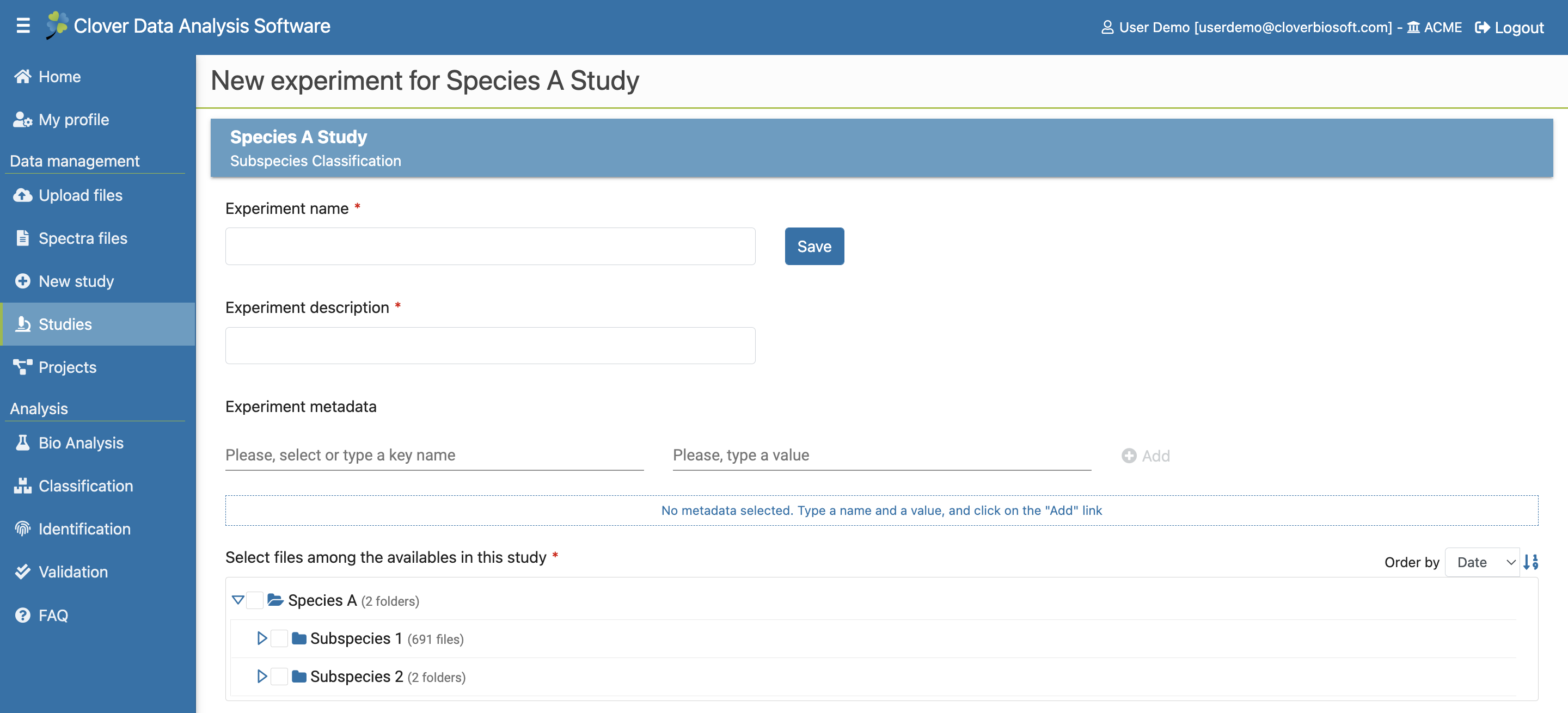
Figure 9.8: New experiment step layout
Please note that only the folders and files that are included in the study will appear here.
Once you have created the experiment, the platform will take you to the experiment layout (Figure 9.9). This experiment will be empty (with no peak matrices and no preprocessing). You must choose then between preprocess the spectra attached to the experiment, or create a new peak matrix. The usual procedure is to apply a preprocessing before creating any peak matrix, thereby, all peak matrices generated after this will be equally preprocessed and their replicates (if applicable) managed. Both processes will be described in detail in Preprocess data process and Peak Matrix Generation process.

Figure 9.9: Empty experiment layout
Please note that only studies created by yourself are susceptible to be deleted.
The third option that you can do without creating a peak matrix or applying any preprocessing is a Biomarker Analysis/Technical analysis. Although a preprocessing with noise reduction applied is always recommended, you can run this analysis with raw data. Either checking how preprocessing affect to your data, making a reproducibility analaysis in a particular point of your replicates or if the preprocessing is already applied by other software. These analysis will be explained in details in Biomarker/Technical Analysis.
9.3. Detailed experiment subsection
If you click on the experiment name in the Detailed study section (Figure 9.3b) its specific experiment section layout displays with all the related information about the selected experiment.
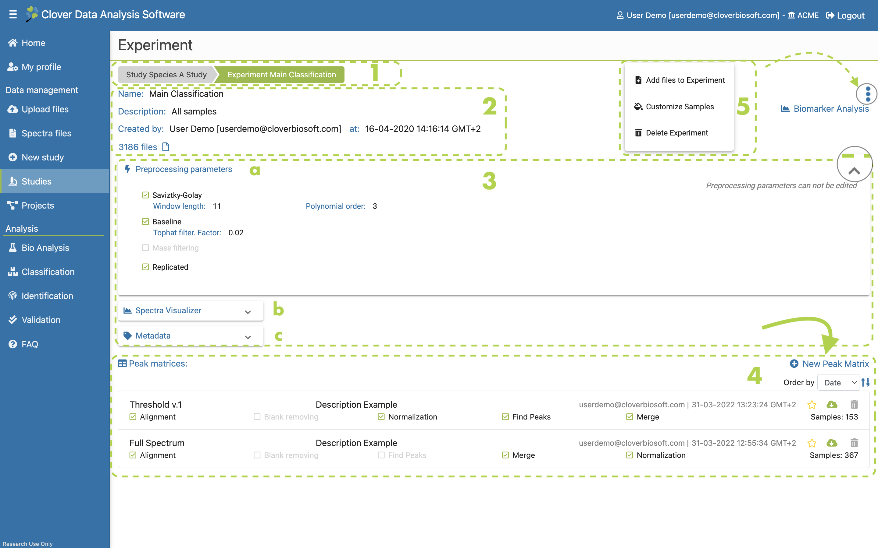
Figure 9.10: Detailed experiment layout with peak matrices